Fundamentals of Network Engineering: Optimizing and Understanding TCP's Behavior - Part 4

Network Address Translation (NAT)

Beyond the basics, TCP’s performance can be significantly impacted by various factors and algorithms. This article explores Network Address Translation, connection states, packet sizing, and two algorithms designed to improve efficiency but which can introduce latency.

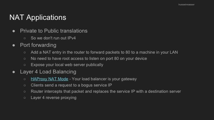
NAT allows multiple devices on a local network to share a single public IP address:

• Maps private IP addresses to public IP addresses
• Essential for IPv4 address conservation
• Creates challenges for certain applications and protocols
• Has implications for direct connectivity between devices

Real-World Implications of TCP Connection States

When a TCP connection closes, both client and server go through several states:

1. The server sends FIN_WAIT_1 to initiate connection closure
2. The client acknowledges and enters CLOSE_WAIT state
3. The client sends its own FIN request and enters LAST_ACK state
4. The server acknowledges and enters TIME_WAIT state, holding resources until confirmation

This state maintenance:

• Consumes memory in server file descriptors
• Keeps connections open even after logical closure
• Can impact server performance during high-volume connection handling

An optimization involves having clients initiate closure requests, preventing servers from entering the TIME_WAIT state.

TCP Advantages:

• Guarantee delivery
• No one can send data without prior knowledge
• Flow Control and Congestion Control
• Ordered Packets no corruption or app level work
• Secure and can’t be easily spoofed

TCP Disadvantages:

• Large header overhead compared to UDP
• More bandwidth
• Stateful - consumes memory on server and client
• Considered high latency for certain workloads (Slow start/ congestion/ acks)
• Does too much at a low level (hence QUIC)
• Single connection to send multiple streams of data (HTTP requests)
• Stream 1 has nothing to do with Stream 2
• Both Stream 1 and Stream 2 packets must arrive
• TCP Meltdown
• Not a good candidate for VPN

MSS/MTU and Path MTU: Understanding Packet Size Limitations

One of the fundamental challenges in networking is determining how large data packets can be:

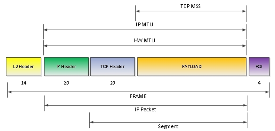
The Layering of Network Units

• TCP (Layer 4): Data is organized into segments
• IP (Layer 3): Segments are encapsulated into packets with headers
• Data Link (Layer 2): Packets are placed into frames

The critical constraint: The frame size is fixed based on network configuration, which ultimately determines segment size.

Hardware MTU Explained

The Maximum Transmission Unit (MTU) defines the size of a frame:

• It’s a property of the network interface (default is typically 1500 bytes)
• Some networks support “jumbo frames” up to 9000 bytes
• Larger frames can reduce latency by requiring fewer transmissions
• However, larger frames are more vulnerable to corruption on unstable networks

IP Packets and MTU Relationship

• IP MTU typically equals the hardware MTU
• Ideally, one IP packet should fit within a single frame
• If necessary, IP fragmentation splits large packets into multiple frames
• Fragmentation can impact performance

Maximum Segment Size (MSS)

MSS is calculated based on the MTU:

MSS = MTU - IP Headers - TCP Headers

Using standard values: MSS = 1500 - 20 - 20 = 1460 bytes

This means:

• A 1460-byte payload fits perfectly in one MSS
• Which fits in one IP packet
• Which fits in one frame
• Resulting in optimal transmission efficiency

From: https://learningnetwork.cisco.com/s/question/0D53i00000Kt7CXCAZ/mtu-vs-pdu

Summary of MTU and MSS Concepts:

• MTU is the maximum transmission unit at the device level
• MSS is the maximum segment size at layer 4
• Larger segments reduce latency and overhead
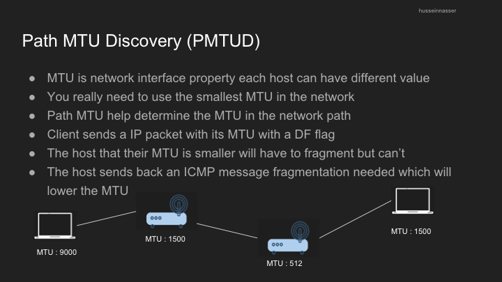
• Path MTU discovery finds the lowest MTU along a network path using ICMP
• Flow and congestion control mechanisms still allow multiple segments to be sent before acknowledgment

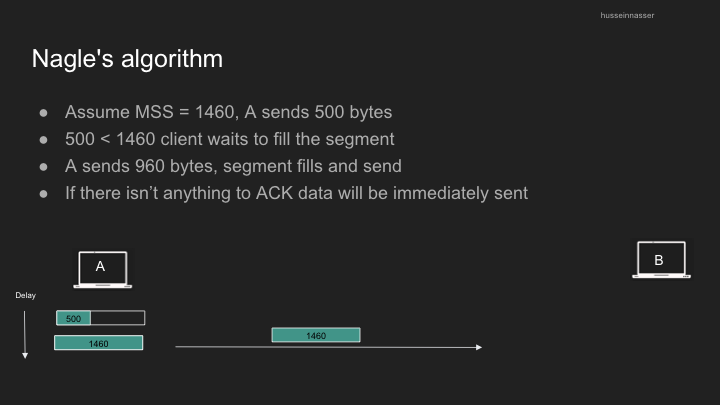
Nagle’s Algorithm: Efficiency vs. Latency

Nagle’s algorithm was designed to improve network efficiency by reducing the number of small packets sent:

• Origin: Created during the telnet era when sending single bytes was common
• Purpose: Combines small segments into single, larger ones
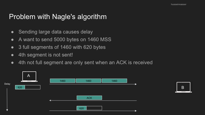
• Function: Client waits until it has a full MSS before sending, or until all previous segments are acknowledged
• Benefit: Reduces wasted bandwidth from 40-byte headers (IP + TCP) carrying only a few bytes of actual data
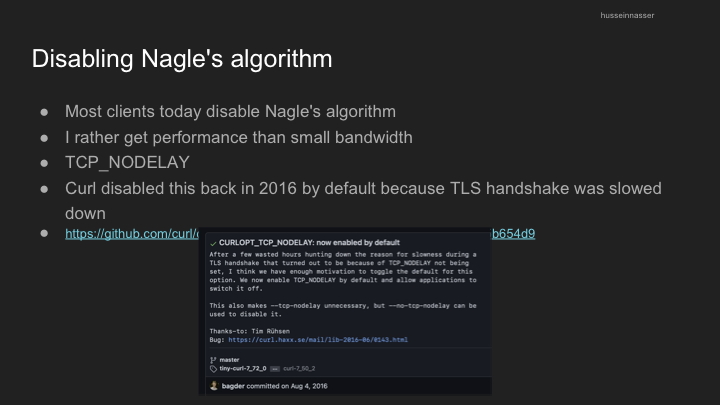
• Trade-off: Can introduce delays, especially in TLS communications
• Real-world impact: Applications like Curl has disabled this feature as it started observing delay in TLS as Nagle’s algo expect packet to be completely filled before sending it until acknowledgement is received. This wait is viewed as delay or performance lag.

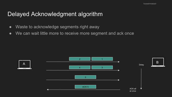
Delayed Acknowledgement

Similar to Nagle’s algorithm, delayed acknowledgment aims to reduce packet overhead:

• Receivers don’t immediately acknowledge every segment
• Instead, they wait for either:
  • Another segment to arrive (allowing one ACK to cover two segments)
  • A timeout (typically 200-500ms)

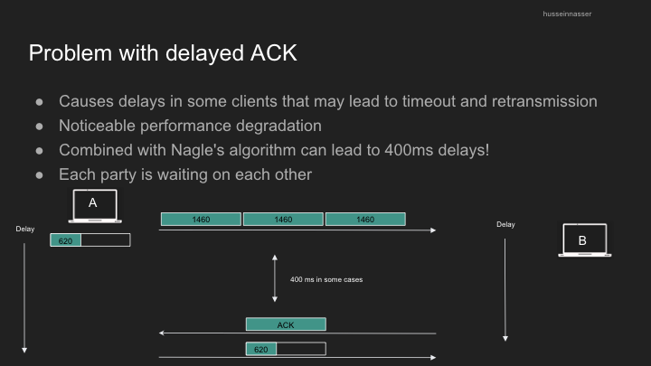
While this reduces network traffic, it can cause performance issues when combined with Nagle’s algorithm, creating a “mini-deadlock” situation where both sides are waiting for the other.

You can disable delayed acknowledgments using the TCP_QUICKACK option, making segments acknowledge faster at the cost of additional network traffic. Segments will be acknowledged “quicker”

previous part

continue to next part

This blog post was compiled from my notes on a Networking Fundamentals course. I hope it helps clarify these essential concepts for you!