Part 1: Database Engineering Fundamentals

Table of Contents

• ACID Properties
• Understanding Database Internals
• Row-Based vs Column-Based Databases
• Primary Key vs Secondary Key
• Database Indexing
• SQL Query Planner and Optimizer
• Scan Types
• Key vs Non-key Column Database Indexing
• Index Scan vs Index Only Scan
• Combining Database Indexes
• Database Optimizer Decisions
• Creating Indexes Concurrently
• Bloom Filters
• Working with Billion Row Tables
• Articles

---

ACID Properties

What is a transaction?

• A collection of queries
• One unit of work
• Example: Select, Update, Update
• Lifespan:
  • Transaction BEGIN
  • Transaction COMMIT
  • Transaction ROLLBACK
  • Transaction unexpected ending → ROLLBACK

Different databases try to optimize operations like rollback or commit. In Postgres, commit I/O is more frequent and commit is faster.

Nature of transactions

• Usually transactions are used to change and modify data
• However, it is perfectly normal to have a read-only transaction
• Example: You want to generate a report and you want to get a consistent snapshot based at the time of transaction
• We will learn more about this in the Isolation section

Atomicity

• All queries in a transaction must succeed
• If one query fails, all prior successful queries in the transaction should rollback
• If the database went down prior to a commit of a transaction, all the successful queries in the transaction should rollback
• After we restart the machine, the first account has been debited but the other account has not been credited
• This is really bad as we just lost data, and the information is inconsistent
• An atomic transaction is a transaction that will rollback all queries if one or more queries failed
• The database should clean this up after restart

Some databases don’t allow operations unless rollback is completed. For long transactions, it can take longer time (like 1 hour) to rollback.

Isolation

• Can my inflight transaction see changes made by other transactions?
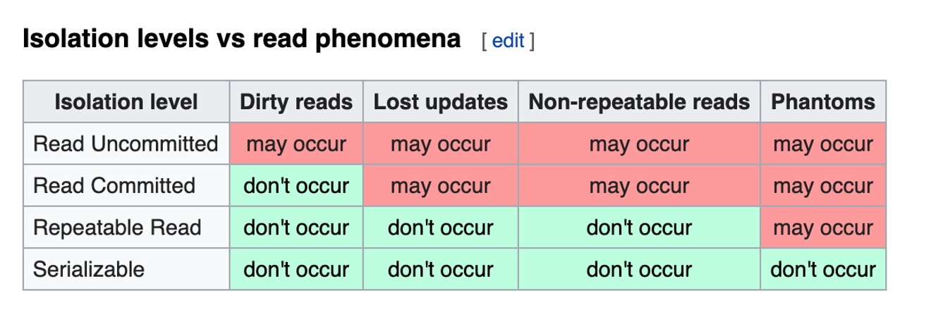
• Read phenomena
• Isolation Levels

Isolation - Read phenomena

• Dirty reads: Reading uncommitted data
• Non-repeatable reads: In a transaction, execution of the same read query results in different values at different times. It is expensive to undo. The value read is committed value but that happened during transaction
• Phantom reads: You are reading data which did not exist at the beginning of the transaction but got committed by another transaction in between. This data is read by a subsequent query
• Lost updates: Two transactions reading the same data and updating it in parallel. The update done by the first transaction gets modified by the second transaction. This makes the result inconsistent

Isolation - Levels

• Read uncommitted: No isolation, any change from the outside is visible to the transaction, committed or not
• Read committed: Each query in a transaction only sees committed changes by other transactions
• Repeatable Read: The transaction will make sure that when a query reads a row, that row will remain unchanged while it’s running. (In Postgres, it is called snapshot isolation, it is versioned)
• Snapshot: Each query in a transaction only sees changes that have been committed up to the start of the transaction. It’s like a snapshot version of the database at that moment
• Serializable: Transactions are run as if they were serialized one after the other

• Each DBMS implements isolation levels differently
• Pessimistic: Row level locks, table locks, page locks to avoid lost updates
• Optimistic: No locks, just track if things changed and fail the transaction if so
• Repeatable read “locks” the rows it reads but it could be expensive if you read a lot of rows; Postgres implements RR as snapshot. That is why you don’t get phantom reads with Postgres in repeatable read
• Serializable are usually implemented with optimistic concurrency control, you can implement it pessimistically with SELECT FOR UPDATE

---

Understanding Database Internals

How tables and indexes are stored on disk

Storage concepts:

• Table
• Row_id
• Page
• IO
• Heap data structure
• Index data structure b-tree
• Example of a query

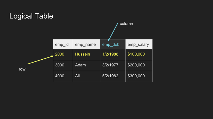
Logical Table

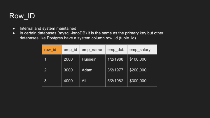
Row_ID

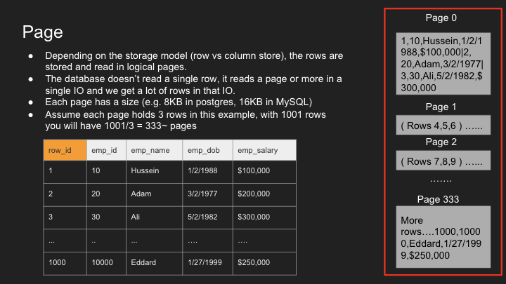
Page

IO

• IO operation (input/output) is a read request to the disk
• We try to minimize this as much as possible
• An IO can fetch 1 page or more depending on the disk partitions and other factors
• An IO cannot read a single row; it’s a page with many rows in them, you get them for free
• You want to minimize the number of IOs as they are expensive
• Some IOs in operating systems go to the operating system cache and not disk

Heap

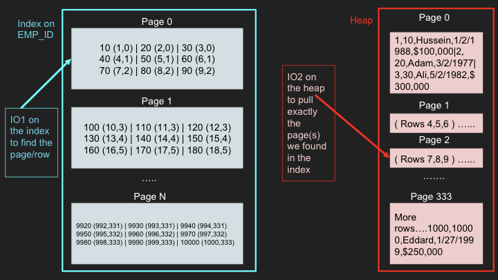
• The Heap is a data structure where the table is stored with all its pages one after another
• This is where the actual data is stored including everything
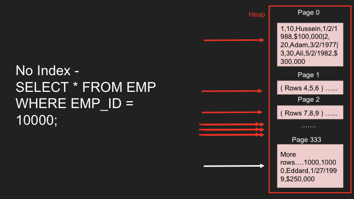
• Traversing the heap is expensive as we need to read so much data to find what we want
• That is why we need indexes that help tell us exactly what part of the heap we need to read, which page(s) of the heap we need to pull

Index

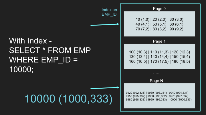
• An index is another data structure separate from the heap that has “pointers” to the heap
• It has part of the data and is used to quickly search for something
• You can index on one column or more
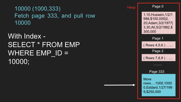
• Once you find a value of the index, you go to the heap to fetch more information where everything is stored
• Index tells you EXACTLY which page to fetch in the heap instead of taking the hit to scan every page in the heap
• The index is also stored as pages and costs IO to pull the entries of the index
• The smaller the index, the more it can fit in memory, and the faster the search
• Popular data structure for index is b-trees, learn more on that in the b-tree section

Notes:

• Sometimes the heap table can be organized around a single index. This is called a clustered index or an Index Organized Table
• Primary key is usually a clustered index unless otherwise specified
• MySQL InnoDB always has a primary key (clustered index); other indexes point to the primary key “value”
• Postgres only has secondary indexes and all indexes point directly to the row_id which lives in the heap

---

Row-Based vs Column-Based Databases

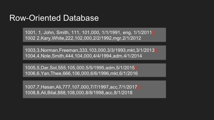
In row-based databases, data is organized in a continuous sequence of bytes which contains all columns of the row together. When a record is fetched, the whole page is returned which contains a number of rows including the one that the query is made for.

• Tables are stored as rows in disk
• A single block IO read to the table fetches multiple rows with all their columns
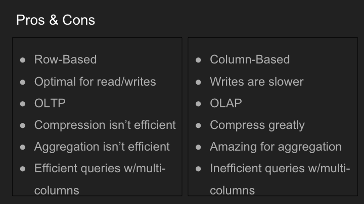
• More IOs are required to find a particular row in a table scan but once you find the row, you get all columns for that row

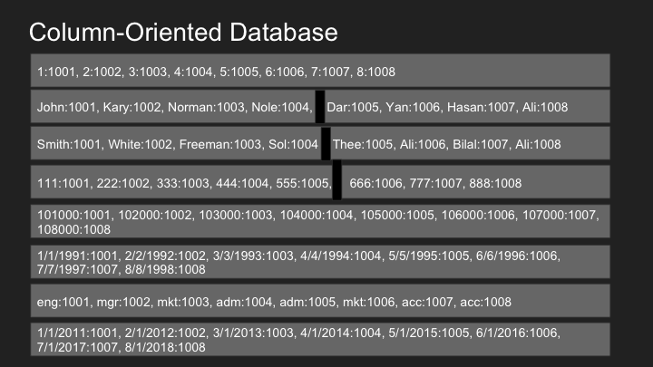
For column-based databases, columns are stored separately where column 1 of all records will be together and the same for all other columns.

• Tables are stored as columns first in disk
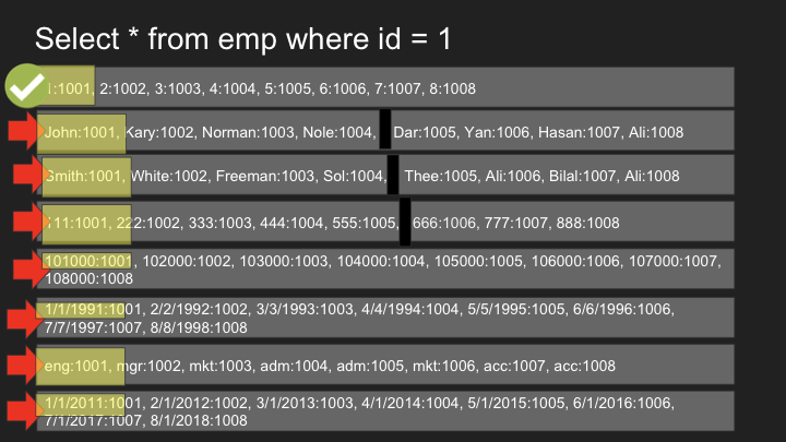
• A single block IO read to the table fetches multiple columns with all matching rows
• Less IOs are required to get more values of a given column. But working with multiple columns requires more IOs
• Typically used for OLAP workloads

---

Primary Key vs Secondary Key

Clustering - organizing a table around a key → Primary key (Oracle and MySQL offer this)

A cluster is nothing but a heap → it is designed for speed for operations like range searches in one IO.

Secondary key → having an additional index in the form of a btree. It has a separate structure from the order in which data is stored. It has row_id as a reference, which is used to locate the actual data.

All indexes in Postgres are secondary indexes.

---

Database Indexing

To check query execution strategy: explain analyze select id from employees e where e.id = 20000;

To create an index: create index <index_name> on table(column_name);

create table employees( id serial primary key, name text);

create or replace function random_string(length integer) returns text as 
$$
declare
  chars text[] := '{0,1,2,3,4,5,6,7,8,9,A,B,C,D,E,F,G,H,I,J,K,L,M,N,O,P,Q,R,S,T,U,V,W,X,Y,Z,a,b,c,d,e,f,g,h,i,j,k,l,m,n,o,p,q,r,s,t,u,v,w,x,y,z}';
  result text := '';
  i integer := 0;
  length2 integer := (select trunc(random() * length + 1));
begin
  if length2 < 0 then
    raise exception 'Given length cannot be less than 0';
  end if;
  for i in 1..length2 loop
    result := result || chars[1+random()*(array_length(chars, 1)-1)];
  end loop;
  return result;
end;
$$ language plpgsql;

insert into employees(name)(select random_string(10) from generate_series(0, 1000000));

create index employees_name on employees(name);

Query: explain analyze select id,name from employees e where e.name like ‘%Pra%’;

Output:

Scan type:
---
- inline index scan → when details present in index, it will not check table/heap
Index Only Scan using employees_pkey on employees e  (cost=0.42..8.44 rows=1 width=4) (actual time=0.051..0.082 rows=1 loops=1)
Index Cond: (id = 20000)
Heap Fetches: 1
Planning Time: 0.241 ms
Execution Time: 0.178 ms
- parallel sequencial  scan → when using non index column to search
Gather  (cost=1000.00..11310.94 rows=6 width=10) (actual time=57.742..64.152 rows=0 loops=1)
Workers Planned: 2
Workers Launched: 2
->  Parallel Seq Scan on employees e  (cost=0.00..10310.34 rows=2 width=10) (actual time=30.379..30.398 rows=0 loops=3)
Filter: (name = 'Pravin'::text)
Rows Removed by Filter: 333334
Planning Time: 0.159 ms
Execution Time: 64.236 ms
- Bitmap index scan → when using index column to search
create index using → **create** **index** employees_name **on** employees(**name**); → this takes time as it build the b tree before using it. if we run same query like above, it will return in lesser time.
Bitmap Heap Scan on employees e  (cost=4.47..27.93 rows=6 width=10) (actual time=0.113..0.160 rows=0 loops=1)
Recheck Cond: (name = 'Pravin'::text)
->  Bitmap Index Scan on employees_name  (cost=0.00..4.47 rows=6 width=0) (actual time=0.052..0.068 rows=0 loops=1)
Index Cond: (name = 'Pravin'::text)
Planning Time: 0.416 ms
Execution Time: 0.261 ms
if we use query that has like usage, it make the DB to check all the rows.
Gather  (cost=1000.00..11319.34 rows=90 width=10) (actual time=6.080..66.693 rows=19 loops=1)
Workers Planned: 2
Workers Launched: 2
->  Parallel Seq Scan on employees e  (cost=0.00..10310.34 rows=38 width=10) (actual time=15.069..42.456 rows=6 loops=3)
Filter: (name ~~ '%Pra%'::text)
Rows Removed by Filter: 333327
Planning Time: 3.247 ms
Execution Time: 67.227 ms
Using explain analyze, we can come to know why query is slower possibly it is using parallel seq scan despite presence of index. so like query is bad query for index.

---

SQL Query Planner and Optimizer

create table grades (
  id serial primary key, 
  g int,
  name text 
); 
create index grades_score on grades(g);

insert into grades (g, name) select random()*100, substring(md5(random()::text ),0,floor(random()*31)::int) from generate_series(0, 500);
vacuum (analyze, verbose, full);

explain analyze select id,g from grades where g > 80 and g < 95 order by g;

explain this keyword is used to check what planning the database will use.

explain select * from grades;

The output is:

Seq Scan on grades  (cost=0.00..75859.70 rows=4218170 width=23)

• cost=0.00..75859.7 → here the first part means, the database took no time to find the first record. As we scan the next record, this time will increase and that is what the database is showing in the second part where it says that the estimate is around 75859.7 ms.
• rows=4218170 → this is just a guess number as the database has not executed the query yet. It is the fastest approach and can be used to replace count(*). In most usecase, you want to show a close-to-exact number which the above query does very efficiently.
• width=23, it is in bytes and represents result size.

Let’s spice it up a bit:

explain select * from grades order by g;

It returns:

Index Scan using grades_score on grades  (cost=0.43..226671.63 rows=5000502 width=23)

Here, the database will use an index scan. It says it will take a cost of .43 ms as something more is going on here. The rows scanned it shows higher.

If you try to sort based on a non-index column:

explain select * from grades order by name;

Here is the output:

Gather Merge  (cost=359650.50..845844.25 rows=4167084 width=23)
  Workers Planned: 2
  ->  Sort  (cost=358650.48..363859.33 rows=2083542 width=23)
        Sort Key: name
        ->  Parallel Seq Scan on grades  (cost=0.00..54513.43 rows=2083542 width=23)

---

Scan Types

Sequential Scan vs Index Scan vs Bitmap Index Scan

All 3 are different scan types that the database uses to retrieve records.

Index scan → If the database finds that the number of records is few, it uses Index scan. In index scan, it uses both the index and heap to retrieve the record.

explain select name from grades where g > 100;
Index Scan using grades_score on grades  (cost=0.43..8.45 rows=1 width=15)
  Index Cond: (g > 100)

You can see the number of rows fetched is small.

Sequential scan → If the database finds that the number of records is large, it will use Sequential scan instead of Index scan. It simply uses Sequential scan and avoids referring to the index to scan the record as there is too much overhead and it slows the performance. The database uses a smart approach here.

explain select name from grades where g < 100;

Seq Scan on grades  (cost=0.00..96184.27 rows=4977500 width=15)
  Filter: (g < 100)

You can see the number of rows fetched is very high, so it uses Sequential scan.

In Bitmap scan there are 3 things happening:

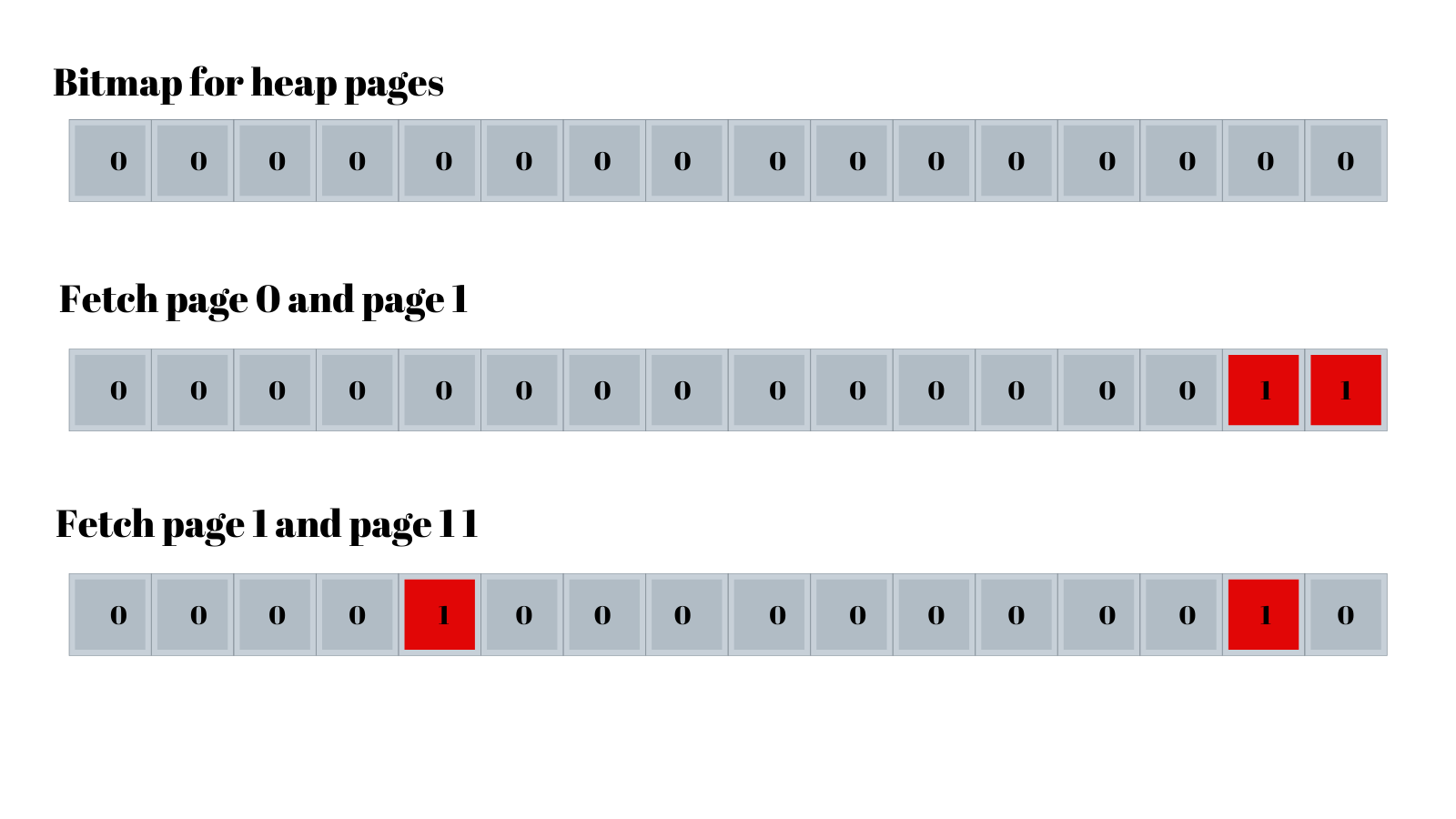
• Bitmap index scan → It first scans the index for grades that are more than 95, it will not visit the heap yet. It will mark the pages that contain the required index.

• Bitmap Heap scan → Once index scan is completed, it will now scan the heap and look for all the pages in the heap. The heap returns the pages which contain more rows, and can have rows which don’t have grade greater than 95. In the next step it performs recheck.
• Recheck index condition → This step applies the final filter to pick the required rows and discard others.

explain select name from grades where g > 95;

Bitmap Heap Scan on grades  (cost=2177.00..38294.62 rows=195170 width=15)
  Recheck Cond: (g > 95)
  ->  Bitmap Index Scan on grades_score  (cost=0.00..2128.21 rows=195170 width=0)
        Index Cond: (g > 95)

Let’s take another example where we’re adding another condition for id < 10,000:

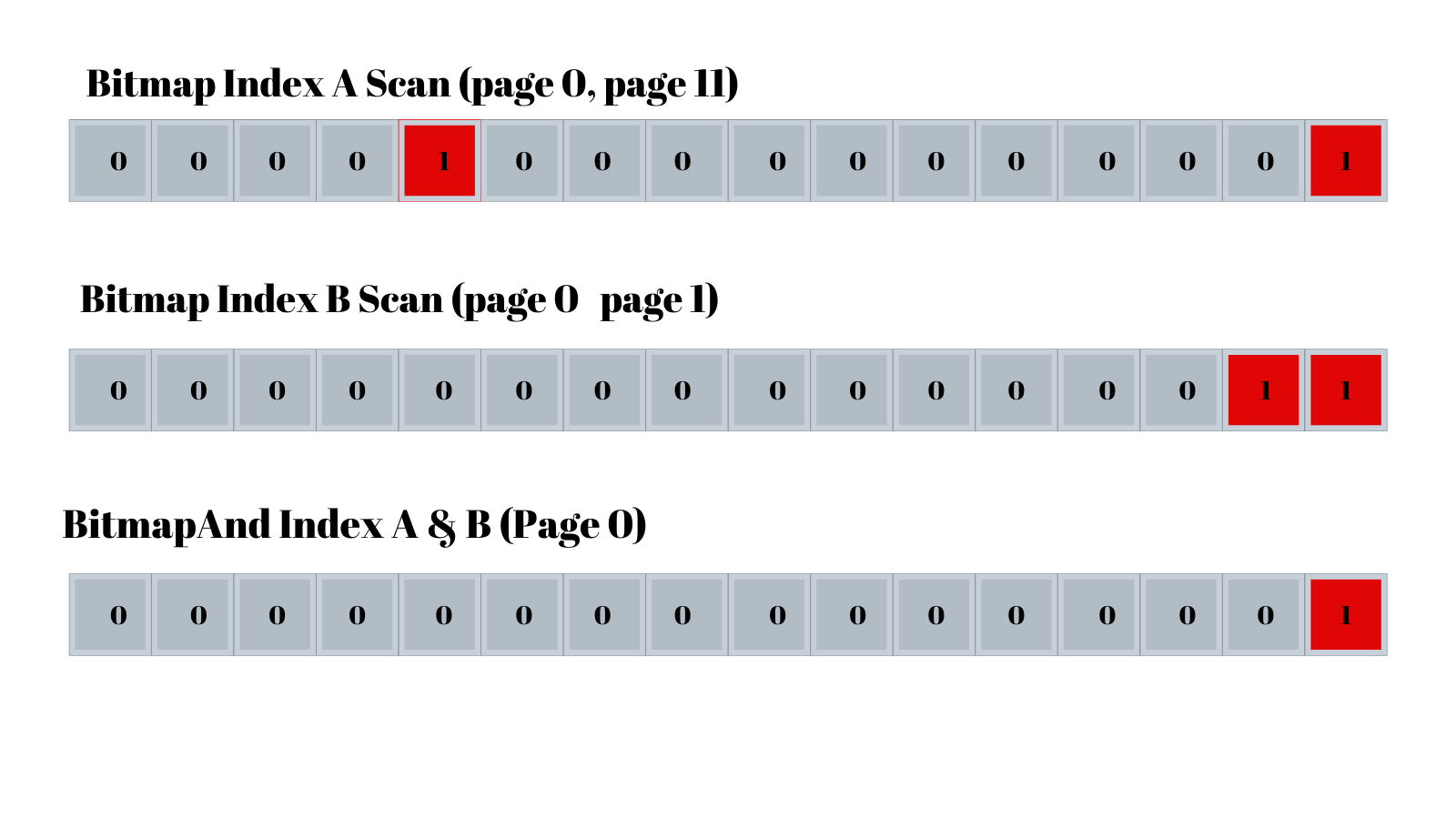
There will be an index scan that will happen for the id column where it will mark pages that have ids less than 10000, and another bitmap index scan happens for pages that contain grades > 95. Later the result from both scans undergoes a bitwise AND operation and is returned for page retrieval from Bitmap heap scan. The same can be understood from the diagram below:

explain select name from grades where g > 95 and id > 10000;

Bitmap Heap Scan on grades  (cost=3988.96..5479.62 rows=394 width=4)
  Recheck Cond: ((g > 95) AND (id < 10000))
  -> BitmapAnd (cost=3988.96..3988.96 rows=394 width=0)
      ->  Bitmap Index Scan on grades_score  (cost=0.00..180.21 rows=9570 width=0)
            Index Cond: (g > 95)
      ->  Bitmap Index Scan on grades_pkey  (cost=0.00..3803.31 rows=195170 width=0)
            Index Cond: (id < 10000)

Key vs Non-key Column Database Indexing

Let’s understand using an example to see performance when data is added in index vs not in index.

For a table created using this script:

create table students (
  id serial primary key, 
  g int,
  firstname text, 
  lastname text, 
  middlename text,
  address text,
  bio text,
  dob date,
  id1 int,
  id2 int,
  id3 int,
  id4 int,
  id5 int,
  id6 int,
  id7 int,
  id8 int,
  id9 int
); 

insert into students (g,
  firstname, 
  lastname, 
  middlename,
  address,
  bio,
  dob,
  id1,
  id2,
  id3,
  id4,
  id5,
  id6,
  id7,
  id8,
  id9) 
select 
  random()*100,
  substring(md5(random()::text ),0,floor(random()*31)::int),
  substring(md5(random()::text ),0,floor(random()*31)::int),
  substring(md5(random()::text ),0,floor(random()*31)::int),
  substring(md5(random()::text ),0,floor(random()*31)::int),
  substring(md5(random()::text ),0,floor(random()*31)::int),
  now(),
  random()*100000,
  random()*100000,
  random()*100000,
  random()*100000,
  random()*100000,
  random()*100000,
  random()*100000,
  random()*100000,
  random()*100000
from generate_series(0, 5000000);

vacuum (analyze, verbose, full);

Result of this query:

explain analyze select id,g from students where g > 80 and g < 95 order by g;

The output shows:

Gather Merge  (cost=157048.00..223006.83 rows=565322 width=8) (actual time=6018.645..21020.085 rows=700746 loops=1)
  Workers Planned: 2
  Workers Launched: 2
  ->  Sort  (cost=156047.97..156754.63 rows=282661 width=8) (actual time=5979.320..8942.869 rows=233582 loops=3)
        Sort Key: g
        Sort Method: external merge  Disk: 4136kB
        Worker 0:  Sort Method: external merge  Disk: 4128kB
        Worker 1:  Sort Method: external merge  Disk: 4120kB
        ->  Parallel Seq Scan on students  (cost=0.00..126587.34 rows=282661 width=8) (actual time=4.775..3025.051 rows=233582 loops=3)
              Filter: ((g > 80) AND (g < 95))
              Rows Removed by Filter: 1433085
Planning Time: 0.138 ms
JIT:
  Functions: 12
  Options: Inlining false, Optimization false, Expressions true, Deforming true
  Timing: Generation 0.986 ms, Inlining 0.000 ms, Optimization 0.717 ms, Emission 13.269 ms, Total 14.972 ms
Execution Time: 29755.348 ms

As we can see, the query is very slow for 5 million records. Now let’s create an index on the g column:

create index g_idx on students(g);

Now if we run the query again:

explain analyze select id,g from students where g > 80 and g < 95 order by g;

The output is:

Gather Merge  (cost=157015.38..222971.41 rows=565298 width=8) (actual time=5943.602..20992.052 rows=700746 loops=1)
  Workers Planned: 2
  Workers Launched: 2
  ->  Sort  (cost=156015.35..156721.97 rows=282649 width=8) (actual time=5906.640..8890.320 rows=233582 loops=3)
        Sort Key: g
        Sort Method: external merge  Disk: 4128kB
        Worker 0:  Sort Method: external merge  Disk: 4128kB
        Worker 1:  Sort Method: external merge  Disk: 4128kB
        ->  Parallel Bitmap Heap Scan on students  (cost=9253.60..126555.89 rows=282649 width=8) (actual time=64.650..3006.930 rows=233582 loops=3)
              Recheck Cond: ((g > 80) AND (g < 95))
              Rows Removed by Index Recheck: 494862
              Heap Blocks: exact=20568 lossy=11260
              ->  Bitmap Index Scan on g_idx  (cost=0.00..9084.01 rows=678358 width=0) (actual time=66.808..66.819 rows=700746 loops=1)
                    Index Cond: ((g > 80) AND (g < 95))
Planning Time: 0.378 ms
JIT:
  Functions: 12
  Options: Inlining false, Optimization false, Expressions true, Deforming true
  Timing: Generation 1.021 ms, Inlining 0.000 ms, Optimization 0.769 ms, Emission 13.504 ms, Total 15.294 ms
Execution Time: 29852.581 ms

Normally anyone would expect the query to be faster now that we’re using an index, but the execution time is still the same or increased a little bit.

One theory is that previously the database was looking only in the table, but now it is looking in the table plus at the primary key index id to retrieve the fields.

Using this command we can determine whether a query is using buffer/cached data and for how many records:

explain (analyze,buffers) select id,g from students where g > 80 and g < 95 order by g desc limit 1000;

Output:

Limit  (cost=0.43..585.94 rows=1000 width=8) (actual time=0.072..51.714 rows=1000 loops=1)
  Buffers: shared hit=782 read=3
  ->  Index Scan Backward using g_idx on students  (cost=0.43..397181.31 rows=678358 width=8) (actual time=0.034..19.658 rows=1000 loops=1)
        Index Cond: ((g > 80) AND (g < 95))
        Buffers: shared hit=782 read=3
Planning:
  Buffers: shared hit=10 read=6
Planning Time: 0.222 ms
Execution Time: 67.558 ms

read=3 → 3 IO operations to disk

Let’s drop the index:

drop index g_idx;

Since we are retrieving id also with grade, let’s include id in the index:

create index g_idx on students(g) include(id);

Now if we run our query:

explain (analyze,buffers) select id,g from students where g > 80 and g < 95;

Output:

Bitmap Heap Scan on students  (cost=14256.95..162273.28 rows=671270 width=8) (actual time=128.376..9821.213 rows=700746 loops=1)
  Recheck Cond: ((g > 80) AND (g < 95))
  Rows Removed by Index Recheck: 1484586
  Heap Blocks: exact=62039 lossy=33262
  Buffers: shared hit=2 read=97217
  ->  Bitmap Index Scan on g_idx  (cost=0.00..14089.13 rows=671270 width=0) (actual time=111.000..111.011 rows=700746 loops=1)
        Index Cond: ((g > 80) AND (g < 95))
        Buffers: shared hit=1 read=1917
Planning:
  Buffers: shared hit=10 read=6
Planning Time: 0.237 ms
JIT:
  Functions: 4
  Options: Inlining false, Optimization false, Expressions true, Deforming true
  Timing: Generation 0.249 ms, Inlining 0.000 ms, Optimization 0.211 ms, Emission 2.586 ms, Total 3.046 ms
Execution Time: 18434.583 ms

We see there is some improvement, but even though id is present in the index, it is not being used and the query planner is using the heap for scanning id. The expectation is that it should not refer to the heap. On repeat queries, it uses cache. High IO means that some part of the index is loaded from disk.

Index Scan vs Index Only Scan

explain analyze select id, name from grades where id = 10000;

Index Scan using grades_pkey on grades  (cost=0.43..8.45 rows=1 width=19) (actual time=0.098..0.135 rows=1 loops=1)
  Index Cond: (id = 10000)
Planning Time: 1.225 ms
Execution Time: 0.246 ms

Here we had an index on the id column, so when we queried using id = it performed an index scan and returned the data.

In this case, first an index lookup happens, then it uses the row_id (internal reference) to fetch the row from the heap. All columns of the row are retrieved, then it picks name and displays it.

explain analyze select id from grades where id = 10000;

Index Only Scan using grades_pkey on grades  (cost=0.43..8.45 rows=1 width=4) (actual time=0.056..0.089 rows=1 loops=1)
  Index Cond: (id = 10000)
  Heap Fetches: 1
Planning Time: 0.077 ms
Execution Time: 0.183 ms

For this query, the DB doesn’t have to lookup the heap to fetch the id as it is already part of the index and it returns that data back. That’s why it’s an Index Only Scan.

If our query somehow uses index only scan then it’s a jackpot as it reduces the response time of the DB to a very low value. One way to use this is to include non-key columns in the index. It is possible to include commonly retrieved data in the index so next time it can use the index.

Here’s an example:

create index id_idx on grades(id) include (name);

explain analyze select id,name from grades where id=1000;

Index Only Scan using id_idx on grades  (cost=0.43..8.45 rows=1 width=19) (actual time=0.036..0.069 rows=1 loops=1)
  Index Cond: (id = 1000)
  Heap Fetches: 1
Planning Time: 0.082 ms
Execution Time: 0.164 ms

Now I am able to retrieve name from the index and avoid lookup from the table.

We need to have a good reason to include non-key columns in an index as it could create more IO operations for index loading once it starts growing larger. Size will become an issue.

Combining Database Indexes for Better Performance

Let’s consider a table:

CREATE TABLE test(
  a INT,
  b INT,
  c TEXT
);

CREATE INDEX a_idx ON test(a);
CREATE INDEX b_idx ON test(b);

Query Behavior Analysis

Case 1: Simple WHERE Clause

SELECT c FROM test WHERE a = 70;

• Database will use Bitmap index scan to check a=70 in different parts of the page
• Later retrieves all records at once using Bitmap heap scan
• If we add LIMIT (e.g., LIMIT 2), it will use Index scan instead to avoid Bitmap overhead

Case 2: AND Condition

SELECT c FROM test WHERE a = 100 AND b = 100;

• Uses Bitmap Index scan for both a and b separately
• Performs an AND operation on the results
• Returns the final result from the heap

Case 3: OR Condition

SELECT c FROM test WHERE a = 100 OR b = 100;

• Execution time is longer than the AND query
• Performs a union of results from both index scans
• More pages to read due to the OR operation

Composite Index Approach

DROP INDEX a_idx, b_idx;
CREATE INDEX a_b_idx ON test(a,b);

Composite Index Behavior:

• It does better job then doing AND on a and b or search on a but not search on b.
• It is a limitation of Postgres that for a composite key, it will use the index when both column is involved or only left side of the key column (a in our case) but not right side of the key column (b in our case will not use index if queried).
• For b-only queries, PostgreSQL will use a full table scan in parallel.
• If you want have faster scan for b column, you can separate index so in case for query involving b column, it will use index specific for b column.
• The advantage for this approach is, in case of OR operation, DB will use composite index when scanning for rows for a column and use b_idx for b column when scanning for rows for B column.
• It will leverage both index to avoid full table scan.

Best Practice:

• For frequently queried columns, maintain separate indexes
• For OR operations, database will use appropriate indexes for each column
• This approach leverages both indexes to avoid full table scans

Database Optimizer Strategies

Reference: multiple-indexes.pdf

Creating Indexes Concurrently

Standard Index Creation

CREATE INDEX idx ON grade(g);

• Blocks write operations
• Allows read operations
• Makes application partially unusable during creation

Concurrent Index Creation

CREATE INDEX CONCURRENTLY g ON grades(g);

Benefits:

• Allows index creation alongside write operations
• Waits for transaction completion before proceeding
• Application remains fully functional

Drawbacks:

• Slower index creation process
• Will fail if there are constraint violations
• Risk of failure increases as application continues adding records

Bloom Filters

Reference: bloom-filter.pdf

Working with Billion-Row Tables

Approach 1: Brute Force

• Full scan table with parallel workers
• Not practical - database will be very slow

Approach 2: Indexing

• Reduces search from billions to millions of rows
• Significant performance improvement

Approach 3: Partitioning

• Slice table into smaller parts
• Apply indexing to each partition
• Each partition can be replicated across different nodes
• Further narrows down search space

Approach 4: Sharding + Partitioning

• Multiple shards, each with multiple partitions
• Each partition has indexing for efficient searching
• Reduces search space to few thousand records

Last Resort:

• If none of the above works, use MapReduce
• Process all records in parallel

Related Articles

• Article - The Cost of Long running Transactions
• Article - Microsoft SQL Server Clustered Index Design
• Database Page